
Statement 7: Forecasting Performance and Scenario Analysis (continued)
Sensitivity and Scenario Analysis
Small movements in economic forecasts or projections can improve or worsen the underlying cash balance, depending on their impacts on payments and receipts. This in turn can drive changes in gross and net debt. Consideration of particular scenarios and sensitivity analysis demonstrates the potential impact of these changes. This analysis highlights the uncertainties that governments face should risks eventuate — for example, in meeting budget forecasts or fiscal targets.
At the 2015‑16 Budget, the analysis included two economic scenarios covering the two forecast years showing the illustrative impact on the fiscal aggregates.
The analysis presented in the 2016‑17 Budget has been expanded to include four economic scenarios that have impacts over the medium term.
Scenarios 1 and 2 explore the sensitivity of fiscal aggregates to a fall in the terms of trade and a delayed recovery in non‑mining business investment. These risks are outlined in Statement 2.
Scenarios 3 to 6 illustrate the sensitivity of fiscal aggregates to changes in key assumptions underpinning the medium‑term economic projections.
Sensitivity analysis over the forecast period
The following two scenarios provide a rule of thumb indication of the sensitivity of receipts, payments and the underlying cash balance to changes in the economic outlook over the forecast period.
Scenario 1: Fall in the terms of trade
This scenario considers the consequences of a permanent 10 per cent fall in world prices of non‑rural commodity exports through 2016‑17. The price fall is consistent with a fall in the terms of trade of 4¾ per cent and a reduction in nominal GDP of 1 per cent by 2017‑18. The sensitivity analysis shows the flow‑on effects to GDP, the labour market and prices. The impacts in Table 1 are stylised and refer to percentage deviations from the Budget forecast levels.
| Impact after 1 year (2016-17) | Impact after 2 year (2017-18) | |
|---|---|---|
| per cent | per cent | |
| Real GDP | 0 | -¼ |
| GDP defaltor | -½ | -¾ |
| Nominal GDP | -½ | -1 |
| Employment | 0 | -¼ |
| Wages | -¼ | -½ |
| CPI | 0 | -¼ |
| Company profits | -1 ¾ | -3 ¼ |
| Nominal household consumption | 0 | -½ |
Assuming no change in exchange rates or interest rates, the fall in export prices leads directly to lower overall output prices (as measured by the GDP deflator) and lower domestic incomes compared with Budget levels. Lower domestic incomes cause both consumption and investment to fall, resulting in lower real GDP and employment and further falls in wages. The fall in aggregate demand puts downward pressure on domestic prices.
On the receipts side, a fall in nominal GDP reduces tax collections. The largest impact is on company tax receipts as the fall in export income decreases company profits. The impact on company tax is larger in 2017‑18, partly owing to lags in tax collections and a larger impact on company profits in the second year of the scenario period. Lower company profits are assumed to flow through to lower Australian equity prices, therefore reducing capital gains tax from individuals, companies and superannuation funds.
On the payments side, a significant proportion of government expenditure is partially indexed to movements in costs (as reflected in various price and wage indicators). Some forms of expenditure, in particular income support payments, are also driven by the number of beneficiaries.
The overall estimated expenditure on income support payments (including pensions, unemployment benefits and other allowances) increases in both years, reflecting a higher number of unemployment benefit recipients. The increase in spending on unemployment benefits in 2017‑18 is partially offset by reduced expenditure on pensions and allowances reflecting slower growth in benefit rates resulting from lower inflation and wages growth. At the same time other payments linked to inflation fall in line with the reduced growth in prices.
Given these assumptions, the overall impact of the fall in the terms of trade is a decrease in the underlying cash balance of around $2.2 billion in 2016‑17 and around $5.4 billion in 2017‑18 (see Table 2).
| 2016‑17 | 2017‑18 | |
|---|---|---|
| $b | $b | |
| Receipts | ||
| Individuals and other withholding taxes | -0.4 | -1.4 |
| Superannuation fund taxes | 0.0 | -0.1 |
| Company tax | -1.6 | -3.2 |
| Goods and services tax | 0.0 | -0.3 |
| Excise and customs duty | 0.0 | -0.2 |
| Other taxes | -0.1 | -0.2 |
| Total receipts | -2.1 | -5.4 |
| Payments | ||
| Income support | -0.1 | -0.2 |
| Other payments | 0.0 | 0.0 |
| Goods and services tax | 0.0 | 0.3 |
| Total payments | -0.1 | 0.1 |
| Public debt interest | 0.0 | -0.1 |
| Underlying cash balance impact(a) | -2.2 | -5.4 |
(a) Estimated impacts fall within the 70 per cent confidence intervals for years 2016‑17 and 2017‑18, as shown in Charts 8 to 10.
This scenario assumes no change in exchange rates. Under a floating exchange rate, however, a fall in the terms of trade would be expected to lead to a depreciation. This would likely dampen the effects on real GDP, meaning the impact on the fiscal position could be smaller.
Scenario 2: Delayed recovery in non‑mining business investment
This scenario considers the consequences of a weaker outlook for business investment than forecast in the Budget. The scenario involves a 3 and 6 per cent reduction in new business investment in 2016‑17 and 2017‑18 respectively, compared with Budget levels, as a result of a delayed recovery in non‑mining business investment. Under this scenario, the level of non‑mining business investment would be broadly flat over this two‑year period.
Once again, the sensitivity analysis evaluates the flow‑on effects to GDP, the labour market and prices. The impacts in Table 3 are stylised and refer to percentage deviations from the Budget forecast levels.
| Impact after 1 year (2016-17) | Impact after 2 year (2017-18) | |
|---|---|---|
| per cent | per cent | |
| Real GDP | -¼ | -½ |
| GDP defaltor | 0 | -¼ |
| Nominal GDP | -¼ | -¾ |
| Employment | -¼ | -½ |
| Wages | 0 | -¼ |
| CPI | 0 | -¼ |
| Company profits | -1 | -1 ¾ |
| Nominal household consumption | 0 | -½ |
Assuming no change in exchange rates or interest rates, the delayed recovery in non‑mining business investment leads directly to lower real GDP compared with Budget levels and also lower imports. This fall in output depresses employment and, in turn, wages. This results in lower levels of consumption. The fall in aggregate demand puts downward pressure on domestic prices.
On the receipts side, lower nominal GDP results in lower tax collections. The initial impact is largest on corporate profits and company tax. In the second year, the larger impact on wages and consumption is expected to result in a larger reduction to tax receipts from individuals and the goods and services tax.
On the payments side, similar to Scenario 1, overall estimated expenditure on income support payments increases in both years due to a higher number of unemployment benefit recipients. The increase in spending on unemployment benefits in 2017‑18 is partially offset by reduced expenditure on pensions and allowances reflecting lower inflation and wages growth. In addition, other payments linked to inflation fall in line with the reduced growth in prices.
The overall impact of the delayed recovery in non‑mining business investment is a decrease in the underlying cash balance of around $1.5 billion in 2016‑17 and around $3.9 billion in 2017‑18 (see Table 4).
| 2016‑17 | 2017‑18 | |
|---|---|---|
| $b | $b | |
| Receipts | ||
| Individuals and other withholding taxes | -0.4 | -1.4 |
| Superannuation fund taxes | 0.0 | -0.1 |
| Company tax | -0.9 | -1.7 |
| Goods and services tax | 0.0 | -0.3 |
| Excise and customs duty | -0.1 | -0.2 |
| Other taxes | 0.0 | 0.0 |
| Total receipts | -1.4 | -3.7 |
| Payments | ||
| Income support | -0.1 | -0.4 |
| Other payments | 0.0 | 0.0 |
| Goods and services tax | 0.0 | 0.3 |
| Total payments | -0.1 | -0.1 |
| Public debt interest | 0.0 | -0.1 |
| Underlying cash balance impact(a) | -1.5 | -3.9 |
(a) Estimated impacts fall within the 70 per cent confidence intervals for years 2016‑17 and 2017‑18, as shown in Charts 8 to 10.
Sensitivity analysis over the medium term
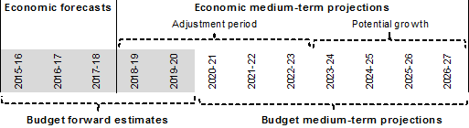
The economic estimates underlying the fiscal projections divide the forecast horizon into a near‑term forecast period and a medium‑term projection period. The forecast period covers the two years following the current financial year. The medium‑term projection period covers the remaining nine years (Chart 11). For the fiscal projections, the medium‑term projection period is the seven years after the Budget forward estimates.
Source: Treasury.
The economic and fiscal projections are not equivalent to the economic and fiscal forecasts. The forecasts are based on a range of short‑run forecasting methodologies informed by professional opinion and information from business liaison. By contrast, the projections are based on a medium‑term methodology. It is crucial to note that they are not estimates or judgments about how conditions will unfold over the medium term. An important assumption is that Government policy does not change.
Economic projections framework
Treasury's medium‑term economic projection methodology assumes that any spare capacity remaining in the economy at the end of the forecast period will be absorbed over the following five years (the adjustment period). Over this period, labour force variables including employment and the participation rate converge to their long‑run trend levels as real GDP returns to potential — the maximum output the economy can produce when there is full employment. This assumption is crucial to the methodology. Importantly, the assumed five‑year timeframe may not be validated and this would affect the projections.
Potential GDP is estimated based on analysis of underlying trends for population, productivity and participation. The Budget forecasts imply that real GDP will be lower than potential GDP at the end of the forecast period — that is, there will be a negative output gap. To close the estimated output gap and absorb forecast spare capacity in the economy, real GDP is projected to grow faster than potential over the adjustment period (over the five years from 2018‑19). By the end of the adjustment period, the output gap is assumed to have closed completely and real GDP grows at its potential rate thereafter.
Fiscal projections framework
Treasury's medium‑term fiscal projections use the Budget forward estimates as a base. They are therefore subject to similar risks and uncertainties that affect the fiscal aggregates discussed earlier in this Statement, but the longer timeframes mean these risks and uncertainties can be amplified.
Beyond the forward estimates, a range of simplifying assumptions are used to project government receipts and payments. The main drivers are movements in economic growth, the size and structure of the population and prices. The medium‑term economic projections are a critical driver of the fiscal projections. For payments, a key parameter is expected per person costs (in each age bracket) of major government programs based on current Government policy. The projections assume current Government policy does not change.
Changes to the assumptions underpinning Treasury's estimate of Australia's potential GDP — as well as the pace of adjustment back to potential — can have large impacts on the fiscal projections. The following section illustrates the sensitivity of fiscal aggregates to these assumptions over the medium‑term projection period.
Output gap scenarios
Scenarios 3 and 4: Alternative output gap adjustment period assumptions
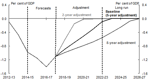
As noted above, the assumption that the adjustment takes five years is crucial and is subject to considerable conjecture as to whether it is appropriate. Scenarios 3 and 4 examine the consequences of shorter (2 years) and longer (8 years) adjustment periods, respectively.
Over the five year adjustment period, real GDP is projected to grow at 3 per cent a year — faster than the estimated potential growth rate of the economy of 2¾ per cent — to close an estimated output gap of around 1 per cent of GDP.
In Scenario 3, a shorter adjustment period requires faster real GDP growth over the adjustment period (Chart 12). In the two‑year adjustment period, annual real GDP growth is 0.3 percentage points higher than in the baseline projections to return the economy to its potential level over two years rather than five years.
Source: Treasury.
| X Values | Short adjustment | Long adjustment | Baseline |
|---|---|---|---|
| 2012-13 | -0.10 | -0.10 | -0.10 |
| 2013-14 | -0.50 | -0.50 | -0.50 |
| 2014-15 | -1.00 | -1.00 | -1.00 |
| 2015-16 | -1.10 | -1.10 | -1.10 |
| 2016-17 | -1.40 | -1.40 | -1.40 |
| 2017-18 | -1.10 | -1.10 | -1.10 |
| 2018-19 | -0.60 | -1.00 | -0.90 |
| 2019-20 | -0.10 | -0.90 | -0.70 |
| 2020-21 | 0.00 | -0.80 | -0.50 |
| 2021-22 | 0.00 | -0.70 | -0.30 |
| 2022-23 | 0.00 | -0.50 | -0.10 |
| 2023-24 | 0.00 | -0.40 | 0.00 |
| 2024-25 | 0.00 | -0.20 | 0.00 |
| 2025-26 | 0.00 | -0.10 | 0.00 |
| 2026-27 | 0.00 | 0.00 | 0.00 |
Under this scenario employment grows more quickly than in the Budget projections, leading to lower unemployment over the first five projection years. This in turn generates faster growth in wages and domestic prices. While the long‑run level of real GDP is unchanged from Budget, the price level is permanently higher. As a result, closing the output gap over two years increases the level of nominal GDP in 2026‑27 by around 1 per cent compared with Budget.
The higher level of nominal GDP also means higher projected tax receipts over the 10‑year period to 2026‑27. Payments are projected to be lower, driven largely by lower projected unemployment which reduces unemployment benefit recipient numbers.
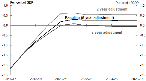
Overall, the faster adjustment in Scenario 3 has a positive impact on the underlying cash balance (Chart 13). In this scenario, the underlying cash balance peaks at 0.6 per cent of GDP in 2020‑21, to be 0.5 per cent of GDP in 2026‑27. This is compared with a peak of 0.3 per cent of GDP in 2021‑22 to be 0.2 per cent of GDP by the end of the medium term in the baseline.
The variation in the underlying cash balance would have implications for the level of government debt. Under Scenario 3, gross debt would be lower, reflecting lower Government borrowing associated with the stronger Budget position. Public debt interest payments would also be lower. This reinforces the improvement in the underlying cash balance.
In Scenario 4, a longer adjustment period requires slower real GDP growth over the adjustment period to return the economy to its potential level over eight years rather than five. This leads to higher unemployment over the eight years of the adjustment period and slower growth in wages and domestic prices compared with the Budget projections.
A slower adjustment in Scenario 4 has a negative impact on the underlying cash balance. Receipts are lower across the period and payments higher overall. In this scenario, the underlying cash balance peaks at 0.1 per cent of GDP in 2021‑22, reaching a small deficit in 2026‑27. Gross debt and public debt interest payments would be higher than in the baseline scenario.
Source: Treasury projections.
| X Values | 2016-17 Budget | 2016-17 Scenario 3 - Short adjustment | 2016-17 Scenario 4 - Long adjustment |
|---|---|---|---|
| 2016-17 | -2.2 | -2.2 | -2.2 |
| 2017-18 | -1.4 | -1.4 | -1.4 |
| 2018-19 | -0.8 | -0.7 | -0.9 |
| 2019-20 | -0.3 | 0.0 | -0.4 |
| 2020-21 | 0.2 | 0.6 | 0.0 |
| 2021-22 | 0.3 | 0.6 | 0.1 |
| 2022-23 | 0.2 | 0.5 | 0.0 |
| 2023-24 | 0.3 | 0.5 | 0.0 |
| 2024-25 | 0.2 | 0.5 | 0.0 |
| 2025-26 | 0.2 | 0.5 | -0.1 |
| 2026-27 | 0.2 | 0.5 | -0.1 |
Productivity scenarios
Scenarios 5 and 6: Alternative trend labour productivity growth assumptions
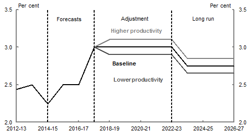
Labour productivity growth is an important determinant of Australia's potential GDP growth. The Budget projections assume that labour productivity grows at a trend rate of 1.6 per cent a year, in line with its 30‑year average annual growth rate.
Scenario 5 examines the consequences of a trend rate of labour productivity growth of 1.5 per cent a year, which is 0.1 percentage points lower than the Budget projections. This reduces the economy's potential growth rate over the projection period (Chart 14). As a result, real GDP grows more slowly over the adjustment period compared with the baseline projections to close the output gap and absorb spare capacity in the economy.
By the end of the projection period in 2026‑27, real GDP is around 1 per cent lower compared with the Budget projections. Lower labour productivity growth also flows through to lower wages. Nominal GDP falls in line with real GDP as there is only a small effect on wages per unit of output (nominal unit labour costs) and, in turn, prices.
Source: ABS cat. no. 5206.0 and Treasury.
| X Values | High productivity | Low productivity | Baseline rounded |
|---|---|---|---|
| 2012-13 | 2.44 | 2.44 | 2.44 |
| 2013-14 | 2.50 | 2.50 | 2.50 |
| 2014-15 | 2.24 | 2.24 | 2.24 |
| 2015-16 | 2.50 | 2.50 | 2.50 |
| 2016-17 | 2.50 | 2.50 | 2.50 |
| 2017-18 | 3.00 | 3.00 | 3.00 |
| 2018-19 | 3.10 | 2.90 | 3.00 |
| 2019-20 | 3.10 | 2.90 | 3.00 |
| 2020-21 | 3.10 | 2.90 | 3.00 |
| 2021-22 | 3.10 | 2.90 | 3.00 |
| 2022-23 | 3.10 | 2.90 | 3.00 |
| 2023-24 | 2.85 | 2.65 | 2.75 |
| 2024-25 | 2.85 | 2.65 | 2.75 |
| 2025-26 | 2.85 | 2.65 | 2.75 |
| 2026-27 | 2.85 | 2.65 | 2.75 |
In Scenario 5, the underlying cash balance peaks at 0.2 per cent of GDP in 2021‑22 before deteriorating to balance by the end of the medium term. This is because of lower projected receipts, owing to lower nominal GDP and a broadly neutral impact on government payments. Gross debt would be higher, reflecting higher borrowing associated with larger Budget deficits. Public debt interest would also be higher.
Scenario 6 assumes a trend labour productivity growth rate of 1.7 per cent a year, which is 0.1 percentage points higher than the assumption factored into the Budget projections. This has broadly opposite effects on the economy compared with Scenario 5, resulting in higher real GDP and higher wages.
In Scenario 6, the underlying cash balance reaches a surplus, peaking at 0.4 per cent of GDP (Chart 15). Gross debt would be lower, reflecting lower Government borrowing. Public debt interest would also be lower.
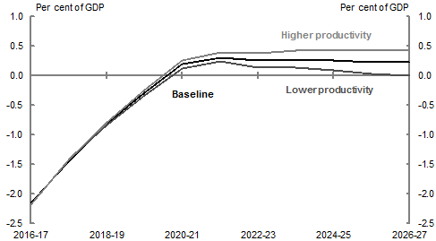
Source: Treasury projections.
| X Values | 2016-17 Budget | 2016-17 Scenario 5 - Low productivity | 2016-17 Scenario 6 - High productivity |
|---|---|---|---|
| 2016-17 | -2.2 | -2.2 | -2.2 |
| 2017-18 | -1.4 | -1.4 | -1.4 |
| 2018-19 | -0.8 | -0.8 | -0.8 |
| 2019-20 | -0.3 | -0.3 | -0.2 |
| 2020-21 | 0.2 | 0.1 | 0.3 |
| 2021-22 | 0.3 | 0.2 | 0.4 |
| 2022-23 | 0.2 | 0.1 | 0.4 |
| 2023-24 | 0.3 | 0.1 | 0.4 |
| 2024-25 | 0.2 | 0.1 | 0.4 |
| 2025-26 | 0.2 | 0.0 | 0.4 |
| 2026-27 | 0.2 | 0.0 | 0.4 |
4 These results represent a partial economic analysis only and do not attempt to capture all the economic feedback and other policy responses related to changed economic conditions, and assume no change in the exchange rate, interest rates or policy over the forecast period.
5 These results represent a partial economic analysis only and do not attempt to capture all the economic feedback and other policy responses related to changed economic conditions, and assume no change in the exchange rate, interest rates or policy over the forecast period.